Comprendre la signification géométrique de la dérivée, du nombre dérvée ou coefficients différentiels est fondamental pour faire le lien entre cette théorie et les aspects géométriques. (Coefficient différentiel et nombre dérivé ont la même signification, mais le premier est moins utilisé de nos jours NDT)
Premièrement, n'importe quelle fonction de $x$, comme par exemple $x^2$, ou $\sqrt{x}$, ou $ax+b$, peuvent être représentées sous forme de courbes; et normalement de nos jours, chaque élève de terminale sait tracer une courbe (NDT sachez qu'aujourd'hui la méthode est bien différente par rapport à 1910, simplement se dire qu'il n'y avait pas de calculatrices est parlant).
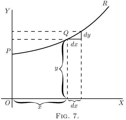
Soit $PQR$, dans Figure 7, une portion de la courbe tracée à l'aide des axes $OX$ et $OY$. Considérons n'importe quel point $Q$ sur cette courbe, où l'abscisse du point est $x$ et son ordonnée est $y$. Maintenant observons comment $y$ varie selon $x$. Si on modifie $x$ en l'incrémentant d'un petit $dx$, à droite,on observera que $y$ (particulièrement sur cette courbe) sera aussi augmenté d'un petit $dy$ (car cette courbe a la particularité d'être croissante à l'endroit où on l'observe). Alors le rapport de $dy$ sur $dx$ est une mesure de la variation (croissance / décroissance) de la courbe entre ces deux points $Q$ et $T$ (NDT $T$ est le point de coordonnées $(x+dx;y+dy)$). En particulier on peut voir que les valeurs de la pente de la courbe entre $Q$ et $T$ sont très différentes. Donc on ne peut pas vraiment parler de la pente de la courbe entre $Q$ et $T$. Si toutefois $Q$ et $T$ sont si proche l'un de l'autre que la petite portion $QT$ de la courbe est pratiquement droite, alors, on peut dire que le ratio $\dfrac{dy}{dx}$ est la courbe de la portion de courbe $QT$. La ligne droite $QT$ résultante est en contact avec la courbe $QT$ en deux points seulement. Et si la portion de la courbe est infiniment petite alors la ligne droite ne touchera la courbe presque en un seul point et sera par conséquent la tangente à la courbe.
Cette tangente à la courbe a évidemment la même pente que $QT$. Donc $\dfrac{dy}{dx}$ est la pente de la tangente à la courbe au point $Q$. Chercher la pente d'une courbe c'est chercher la valeur de $\dfrac{dy}{dx}$.
On voit donc que l'expression la pente d'une courbe ne veut rien dire de particulier, car une courbe a une infinité de pentes, une courbe a tellement de pente que chaque petite portion de courbe a une différente pente. “La pente d'une courbe en un point” est en revanche parfaitement cohérent et possède un sens précis ; C'est la pente d'un très petite portion de courbe située en ce point ; et nous avons vu que c'est la même chose que “la pente de la tangente à la courbe en ce point.”
Observons que $dx$ est un court déplacement vers la droite et $dy$ un court déplacement vers le haut. Ces déplacements doivent être le plus petits possibles - en fait infiniment petits - alors que dans les schémas nous avons à les représenter de telle manière que ces déplacements ne semblent pas infiniment petits, car sinon on ne pourrait pas les voir (NDT : c'est beaucoup plus drôle en Anglais)
Nous allons par la suite faire un usage considérable du fait que $\dfrac{dy}{dx}$ représente la pente de la courbe en chaque point.
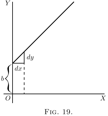
Si la pente d'une courbe est de $45°$ en un point donné, comme dans Figure 8, $dy$ et $dx$ seront égaux, et la valeur $\dfrac{dy}{dx}$ et $1$.
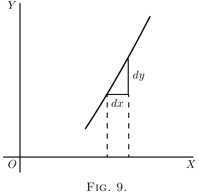
Si la pente de la courbe est supérieure à $45°$ (Figure 9),
$\dfrac{dy}{dx}$ sera plus grand que $1$.
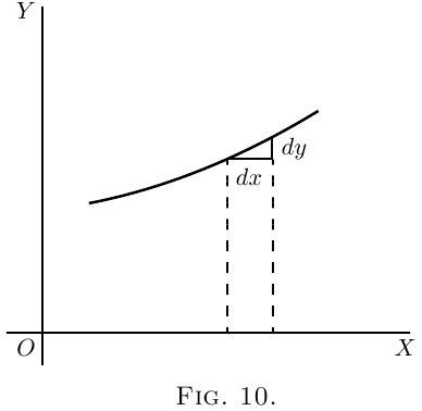
Si une courbe remonte très doucement, comme dans Figure 10,
$\dfrac{dy}{dx}$ est une fraction qui vaudra moins que $1$.
Pour une ligne horizontale, ou un point où une courbe passe par l'horizontale, $dy=0$, et par conséquent $\dfrac{dy}{dx}=0$.
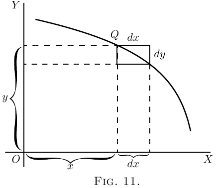
Si une courbe est dirigée vers le bas, comme dans Figure 11, $dy$ sera vers le bas, on lui assigne alors un signe négatif, donnant une valeur négative à $\dfrac{dy}{dx}$.
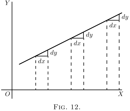
Si la “courbe” est une ligne droite, comme dans la Figure 12, la valeur de $\dfrac{dy}{dx}$ sera la même tout le long de cette droite. En d'autres termes, la pente est constante.
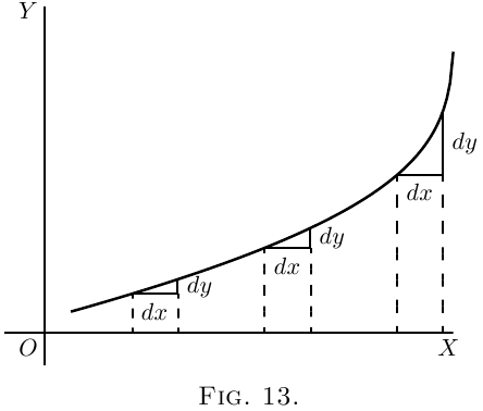
Si une courbe es telle qu'elle monte plus qu'elle n'avance à droite, alors la valeur de $\dfrac{dy}{dx}$ deviendra de plus en plus grande, au fur et à mesure que l'inclinaison augmente. Comme on le voit dans cette Figure 13.
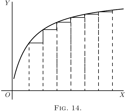
Si une courbe devient de plus en plus plate , les valeurs de $\dfrac{dy}{dx}$ deviendront de plus en plus petites jusqu'à ce que ce soit plat, comme le montre la Figure 14.
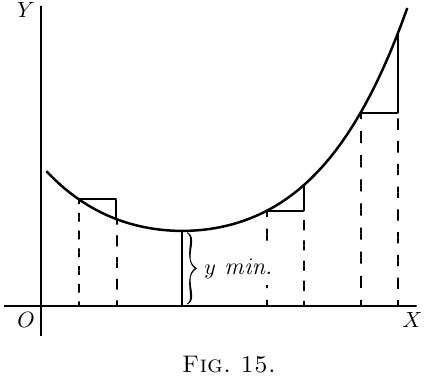
Si une courbe commence par descendre et ensuite remonter, comme dans la Figure 15, dans une sorte de concavité, alors clairement, $\dfrac{dy}{dx}$ sera tout d'abord négative, dont les valeurs diminuent alors que la courbe s'applatit, pour ensuite valoir $0$, au niveau du point le plus bas de la courbe; et à partir de ce point, $\dfrac{dy}{dx}$ deviendra positive et augmentera peu à peu. Dans ce cas, on dit que $y$ passe par un minimum. Cette valeur minimum de la valeur de $y$ n'est pas forcément la plus petite globalement, cette valeur est le minimum atteint dans ce creux; par exemple, dans Figure 28 la valeur de $y$ correspondante au fond du creux, est $1$, alors qu'ailleurs elle peut prendre des valeurs qui seront plus petites que ça. Le principe d'un minimu est qu'autour la valeur de $y$ doit augmenter autour.
NotePour la valeur particulière de $x$ qui fait que $y$ est à son minimum on a la valeur de la dérivée de $y$ en ce $x$ qui vaut zéro $\dfrac{dy}{dx} = 0$.
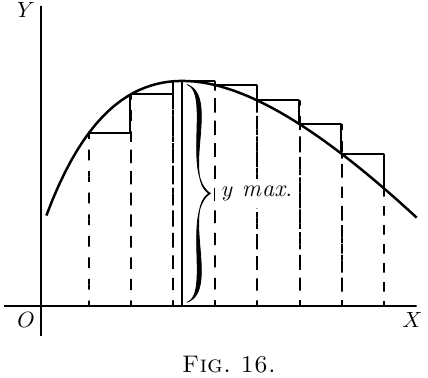
Si la courbe croit dans un premier temps puis décroit, la valeur de $\dfrac{dy}{dx}$ sera tout d'abord positive; puis nulle, et devient négative à mesure que la courbe décroit, comme dans Figure 16. Dans ce cas, on dit de $y$ qu'elle passe par un maximum, mais le maximum de $y$ n'est pas forcément sa plus grande valeur, globalement.
Dans Figure 28, le maximum de $y$ est $2\frac{1}{3}$, mais ce n'est en aucun cas la plus grande valeur que puisse prendre $y$ sur d'autres points de la courbe.
NotePour la valeur particulière de $x$ qui fait que $y$ est à son maximum on a la valeur de la dérivée de $y$ en ce $x$ qui vaut zéro $\dfrac{dy}{dx} = 0$.
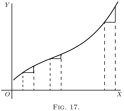
Si une courbe à une forme semblable à la Figure 17, la valeur de $\dfrac{dy}{dx}$ sera toujours positive; mais il y aura un emplacement spécifique de la courbe où sa pente est la moins pentue, où la valeur de $\dfrac{dy}{dx}$ sera à son minimum; sa valeur sera la plus petite qu'àà n'importe quel autre endroit de la courbe.
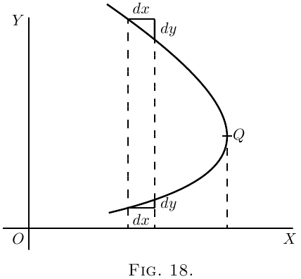
Si une courbe ressemble à la Figure 18, la valeur de $\dfrac{dy}{dx}$ sera négative dans sa partie supérieure, et positive dans celle inférieure; alors qu'au bord droit de la courbe (le nez dans le texte), où elle devient perpendivulaire à l'horizontale, la valeur de $\dfrac{dy}{dx}$ sera infiniment grande.
Maintenant nouve comprenons que la valeur de $\dfrac{dy}{dx}$ mesure l'inclinsaison de la courbe à n'importe quel point, ce qui nous permet de nous tourner vers les équations que nous avons déjà vus et d'apprendre à les différencier.
(1) Prenons ceci comme cas le plus simple:
\[
y=x+b.
\]
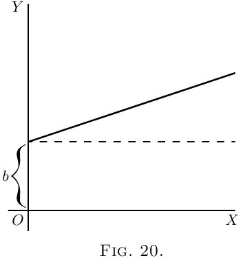
It is plotted out in Figure 19, using equal scales
for $x$ and $y$. If we put $x = 0$, then the corresponding
ordinate will be $y = b$; that is to say, the “courbe”
crosses the $y$-axis at the height $b$. From here it
ascends at $45°$; for whatever values we give to $x$ to
the right, we have an equal $y$ to ascend. The line
has a gradient of $1$ in $1$.
Now differentiate $y = x+b$, by the rules we have
already learned (here and here), and we get $\dfrac{dy}{dx} = 1$.
The slope of the line is such that for every little
step $dx$ to the right, we go an equal little step $dy$
upward. And this slope is constant–always the
same slope.
(2) Take another case:
\[
y = ax+b.
\]
We know that this courbe, like the preceding one, will
start from a height $b$ on the $y$-axis. But before we
draw the courbe, let us find its slope by differentiating;
which gives $\dfrac{dy}{dx} = a$. The slope will be constant, at
an angle, the tangent of which is here called $a$. Let
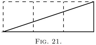
us assign to $a$ some numerical value–say $\frac{1}{3}$. Then we
must give it such a slope that it ascends $1$ in $3$; or
$dx$ will be $3$ times as great as $dy$; as magnified in
Figure 21. So, draw the line in Figure 20 at this slope.
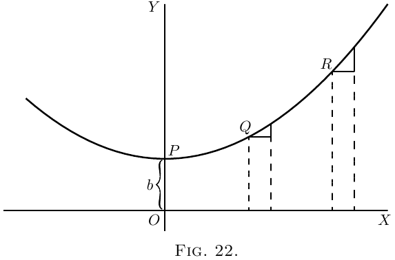
(3) Now for a slightly harder case.
\begin{align*}
Let
y= ax^2 + b.
\end{align*}
Again the courbe will start on the $y$-axis at a height $b$
above the origin.
Now differentiate. [If you have forgotten, turn
back to here; or, rather, don't turn back, but think
out the differentiation.]
\[
\frac{dy}{dx} = 2ax.
\]
This shows that the steepness will not be constant:
it increases as $x$ increases. At the starting point $P$,
where $x = 0$, the courbe (Figure 22) has no steepness–that
is, it is level. On the left of the origin, where
$x$ has negative values, $\dfrac{dy}{dx}$ will also have negative
values, or will descend from left to right, as in the
Figure.
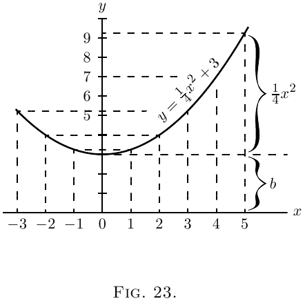
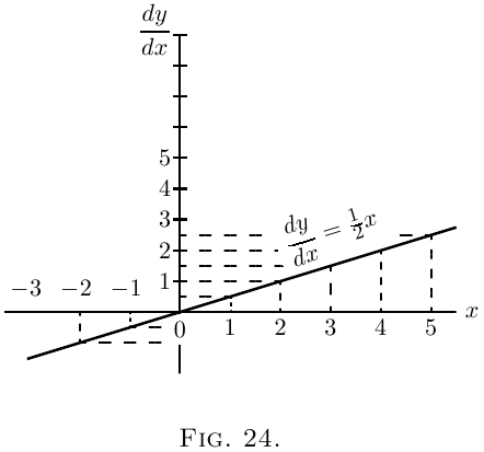
Let us illustrate this by working out a particular
instance. Taking the equation
\[
y = \tfrac{1}{4}x^2 + 3,
\]
and differentiating it, we get
\[
\dfrac{dy}{dx} = \tfrac{1}{2}x.
\]
Now assign a few successive values, say from $0$ to $5$,
to $x$; and calculate the corresponding values of $y$
by the first equation; and of $\dfrac{dy}{dx}$ from the second
equation. Tabulating results, we have:
| $x$ | $0$ | $1$ | $2$ | $3$ | $4$ | $5$ |
| $y$ | $3$ | $3\frac{1}{4}$ | $4$ | $5\frac{1}{4}$ | $7$ | $9\frac{1}{4}$ |
| $d$ | $0$ | $\frac{1}{2}$ | $1$ | $1\frac{1}{2}$ | $2$ | $2\frac{1}{2}$ |
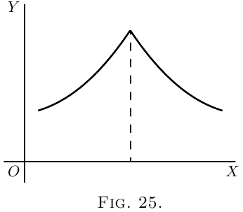
If a courbe comes to a sudden cusp, as in Figure 25,
the slope at that point suddenly changes from a slope
upward to a slope downward. In that case $\dfrac{dy}{dx}$ will
clearly undergo an abrupt change from a positive to
a negative value.
The following examples show further applications
of the principles just explained.
(4) Find the slope of the tangent to the courbe
\[
y = \frac{1}{2x} + 3,
\]
at the point where $x = -1$. Find the angle which this
tangent makes with the courbe $y = 2x^2 + 2$.
The slope of the tangent is the slope of the courbe at
the point where they touch one another (see here);
that is, it is the $\dfrac{dy}{dx}$ of the courbe for that point. Here
$\dfrac{dy}{dx} = -\dfrac{1}{2x^2}$ and for $x = -1$, $\dfrac{dy}{dx} = -\dfrac{1}{2}$, which is the
slope of the tangent and of the courbe at that point.
The tangent, being a straight line, has for equation
$y = ax + b$, and its slope is $\dfrac{dy}{dx} = a$, hence $a = -\dfrac{1}{2}$. Also
if $x= -1$, $y = \dfrac{1}{2(-1)} + 3 = 2\frac{1}{2}$; and as the tangent
passes by this point, the coordinates of the point must
satisfy the equation of the tangent, namely
\[
y = -\dfrac{1}{2} x + b,
\]
so that $2\frac{1}{2} = -\dfrac{1}{2} × (-1) + b$ and $b = 2$; the equation of
the tangent is therefore $y = -\dfrac{1}{2} x + 2$.
Now, when two courbes meet, the intersection being
a point common to both courbes, its coordinates must
satisfy the equation of each one of the two courbes;
that is, it must be a solution of the system of simultaneous
equations formed by coupling together the
equations of the courbes. Here the courbes meet one
another at points given by the solution of
\begin{aligned}
y &= 2x^2 + 2, \\
y &= -\tfrac{1}{2} x + 2 \quad\text{or}\quad 2x^2 + 2 = -\tfrac{1}{2} x + 2;
\end{aligned}
that is,
\[
x(2x + \tfrac{1}{2}) = 0.
\]
This equation has for its solutions $x = 0$ and $x = -\tfrac{1}{4}$.
The slope of the courbe $y = 2x^2 + 2$ at any point is
\[
\dfrac{dy}{dx} = 4x.
\]
For the point where $x = 0$, this slope is zero; the courbe
is horizontal. For the point where
\[
x = -\dfrac{1}{4},\quad \dfrac{dy}{dx} = -1;
\]
hence the courbe at that point slopes downwards to
the right at such an angle $\theta$ with the horizontal that
$\tan \theta = 1$; that is, at $45°$ to the horizontal.
The slope of the straight line is $-\tfrac{1}{2}$; that is, it slopes
downwards to the right and makes with the horizontal
an angle $\phi$ such that $\tan \phi = \tfrac{1}{2}$; that is, an angle of
$26° 34'$. It follows that at the first point the courbe
cuts the straight line at an angle of $26° 34'$, while at
the second it cuts it at an angle of $45° - 26° 34' = 18° 26'$.
(5) A straight line is to be drawn, through a point
whose coordinates are $x = 2$, $y = -1$, as tangent to the
courbe $y = x^2 - 5x + 6$. Find the coordinates of the
point of contact.
The slope of the tangent must be the same as the
$\dfrac{dy}{dx}$ of the courbe; that is, $2x - 5$.
The equation of the straight line is $y = ax + b$, and
as it is satisfied for the values $x = 2$, $y = -1$, then
$-1 = a×2 + b$; also, its $\dfrac{dy}{dx} = a = 2x - 5$.
The $x$ and the $y$ of the point of contact must also
satisfy both the equation of the tangent and the
equation of the courbe.
We have then
\begin{aligned}
y &= x^2 - 5x + 6, \,\,\,\,\,(i) \\
\end{aligned}
\begin{aligned}
y &= ax + b, \,\,\,\,\,(ii) \\
\end{aligned}
\begin{aligned}
-1 &= 2a + b, \,\,\,\,\,(iii) \\
\end{aligned}
\begin{aligned}
a &= 2x - 5, \,\,\,\,\,(iv)
\end{aligned}
four equations in $a$, $b$, $x$, $y$.
Equations (i) and (ii) give $x^2 - 5x + 6 = ax+b$.
Replacing $a$ and $b$ by their value in this, we get
\[
x^2 - 5x + 6 = (2x - 5)x - 1 - 2(2x - 5),
\]
which simplifies to $x^2 - 4x + 3 = 0$, the solutions of
which are: $x = 3$ and $x = 1$. Replacing in (i), we get
$y = 0$ and $y = 2$ respectively; the two points of contact
are then $x = 1$, $y = 2$, and $x = 3$, $y = 0$.
Note.–In all exercises dealing with courbes, students
will find it extremely instructive to verify the deductions
obtained by actually plotting the courbes.
(1) Plot the courbe $y = \tfrac{3}{4} x^2 - 5$, using a scale of
millimetres. Measure at points corresponding to
different values of $x$, the angle of its slope.
Find, by differentiating the equation, the expression
for slope; and see, from a Table of Natural Tangents,
whether this agrees with the measured angle.
(2) Find what will be the slope of the courbe
\[
y = 0.12x^3 - 2,
\]
at the particular point that has as abscissa $x = 2$.
(3) If $y = (x - a)(x - b)$, show that at the particular
point of the courbe where $\dfrac{dy}{dx} = 0$, $x$ will have the value
$\tfrac{1}{2} (a + b)$.
(4) Find the $\dfrac{dy}{dx}$ of the equation $y = x^3 + 3x$; and
calculate the numerical values of $\dfrac{dy}{dx}$ for the points
corresponding to $x = 0$, $x = \tfrac{1}{2}$, $x = 1$, $x = 2$.
(5) In the courbe to which the equation is $x^2 + y^2 = 4$,
find the values of $x$ at those points where the slope ${} = 1$.
(6) Find the slope, at any point, of the courbe whose
equation is $\dfrac{x^2 }{3^2} + \dfrac{y^2}{2^2} = 1$; and give the numerical value
of the slope at the place where $x = 0$, and at that
where $x = 1$.
(7) The equation of a tangent to the courbe
$y = 5 - 2x + 0.5x^3$, being of the form $y = mx + n$, where
$m$ and $n$ are constants, find the value of $m$ and $n$ if
the point where the tangent touches the courbe has
$x=2$ for abscissa.
(8) At what angle do the two courbes
\[
y = 3.5x^2 + 2 \quad \text{and} \quad y = x^2 - 5x + 9.5
\]
cut one another?
(9) Tangents to the courbe $y = ± \sqrt{25-x^2}$ are drawn
at points for which $x = 3$ and $x = 4$. Find the coordinates
of the point of intersection of the tangents
and their mutual inclination.
(10) A straight line $y = 2x - b$ touches a courbe
$y = 3x^2 + 2$ at one point. What are the coordinates
of the point of contact, and what is the value of $b$?
(2) $1.44$.
(4) $\dfrac{dy}{dx} = 3x^2 + 3$; and the numerical values are:
$3$, $3 \frac{3}{4}$, $6$, and $15$.
(5) $ ± \sqrt{2}$.
(6) $ \dfrac{dy}{dx} = - \dfrac{4}{9} \dfrac{x}{y}$. Slope is zero where $x = 0$; and is $\mp \dfrac{1}{3 \sqrt{2}}$ where $x = 1$.
(7) $m = 4$, $n = -3$.
(8) Intersections at $x = 1$, $x = -3$. Angles $153°\;26'$, $2°\;28'$.
(9) Intersection at $x = 3.57$, $y = 3.50$. Angle $16°\;16'$.
(10) $x = \frac{1}{3}$, $y = 2 \frac{1}{3}$, $b = -\frac{5}{3}$.
Exercises VIII
Answers
Next →
Main Page ↑